Draft Minutes

ASC OP1 Optics and Electro-Optical Instruments – Optical Elements and Assemblies – Wavefront Standard

Monday August 27, 2007, 8:30 a.m. – 12:00 noon

Auditor’s Summary of Meeting

At this meeting the task force concentrated upon the statistical evaluation of wavefront measurement. After a presentation about the practical application of power spectral density measurement, D. Aikens presented an edited version of ISO 10110-8 for the Task Force to review as a basis for a new OP1.004 draft document. The document was examined section by section. In the area of surface roughness, much time was devoted to a discussion concerning the designation of power spectral density (PSD) on optical drawings. At the conclusion, it was agreed that there would not be a default specification for PSD, but there would be for rms roughness.

Items that needed definition or description were assigned to various participants, and an interim conference call was planned to report progress before the next meeting in January 2008.

1. Welcome and Introductions

S. Martinek agreed to act as leader of the meeting, and opened the meeting at 8:41a.m. with a round of introductions.

2. Adoption of Agenda

D. Aikens moved to adopt the agenda. M. Dowell seconded the motion, which carried unanimously.

3. Approval of draft minutes of the May 14, 2007 meeting

C. Evans suggested that the term PVr be defined in the minutes because there is no other document that defines it. The secretary asked C. Evans to e-mail the definition to him so that it can be added to the minutes.

PVr has been proposed as a robust PV – which aims to be insensitive to differences in camera pixel resolution and does not require arbitrary removal of "fliers" or spikes.

Definition:

PVr = PV(36 term Zernike fit) + N x rms(Zernike residual)

PVr is the sum of the PV of a 36 term Zernike fit (after removing those terms set to zero (eg piston and tilt for flats) and N times the rms of the residual after fitting to, and removing, 36 terms. The default value of N is 3.

PVr adds a representation of mid-spatial frequency to show that the term is robust for surfaces that follow the type of behavior. It is useful for specifying optics for trade. D. Aikens added that the traditional peak-valley measure has become somewhat obsolete because of modern detector technology. Without specifying some kind of filtering, peak-valley cannot be used. One way to circumvent the problem is to do a Zernike fit to the detector data. The problem of applying Zernikes to the data is that the fitting process does not take into account all of the other Zernike terms that have not been used in the fit. So C. Evans has developed an algorithm that is fairly robust, in that it reports the same value for similarly behaving surfaces. It achieves the spirit of the peak-valley concept, whereby a single number is reported for the surface. The number is different than the corresponding rms value, but it has value, and is much better than the traditional peak-valley reading. V. Yashchuk asked why peak-valley was being specified rather than rms. S. Martinek replied that this provides a link to those in the industry who evaluate surfaces by eye.

D. Aikens moved that the minutes be approved with the addition of the definition of PVr. R. Williamson seconded the motion, which carried unanimously. C. Evans was invited to present a review of PVr at the next meeting.

4. Practical application of power spectrum

J. Harvey showed an example where he was using the surface power spectral density function as a specification for a mirror that was being purchased. Conventionally, figure and finish, or micro-roughness, are specified, such as, figure to be better than 0.1λ and <20 Ǻ rms roughness. The surface power-spectral-density function is essentially a plot of surface variance as a function of spatial frequency. This makes possible the specification of surface irregularity over the entire range of relevant spatial frequencies.

He showed graphs to illustrate an example. The low end of the spatial-frequency domain covers figure errors that produce conventional aberrations, and the high end of the spatial-frequency domain covers micro-roughness that produces the wide-angle scatter that reduces contrast in an image. What has historically not been specified, or measured, is the mid-spatial-frequency surface errors that fall between the conventional figure errors and micro-roughness. When the surface PSD is specified, then the whole range is covered. This technique has been applied to components for a UV telescope. The equation for the PSD is . The resulting curve, which is a radial profile of a 2D PSD, would be the ceiling for acceptance of measured data. Practically, the measured data may wander around the specification curve, and if appropriate, small deviations above the curve in limited areas would be acceptable.

J. Harvey showed graphs comparing predicted and measured BRDF data for a Molybdenum mirror. He stated that they can now use fitted PSD data from measured scatter data to predict the PSD at other wavelengths or angles of incidence.

Fabricators are now being introduced to this method of specification, although there is resistance to using it; however, in time it will become accepted.

Following this presentation, the Task Force took a five minute break.

5. Wavefront Standards

OP1.004

D. Aikens started by saying that P. Takacs had earlier put together a scope statement that lists changes to existing ISO documents required to make a statistically based wavefront standard. D. Aikens took that scope document and used it to review ISO 10110-8. He drafted another document to describe what would need to be changed in order to meet the Takacs scope. D. Aikens presented this latter document at the Paris ISO/TC 172/SC 1 meeting in June. The ISO Working Group accepted the input. There is now a new project to re-author ISO 10110-8 with the US leading the effort.

D. Aikens reminded the group that ISO 10110-8 is only a notation standard; therefore it should not define technical terms. However, in cases where there is no definition elsewhere, terms are defined in it. It will not address measurement.

At this point the the draft was projected for the group to review. The document was also available on the OEOSC web site.

The first change occurred in section 3.5 where new terms were introduced. M. Dowell asked if the terms should be in alphabetical order. D. Aikens said that the existing definitions appeared to be grouped according to the area in the standard that they were being used. If necessary, they can be reordered later. S. Martinek asked if the terms listed in color were terms that D. Aikens had added. D. Aikens confirmed that they were.

C. Evans said that he had been looking in ISO/DIS 25178-2, “Geometrical product specifications (GPS) – Surface texture: Areal – Part 2: Terms, definitions and surface texture parameters.” He said that many of the terms that D. Aikens has added are included there. D. Aikens said that the Task Force has two choices:

1. Make ISO/DIS 25178-2 a normative reference, which means that users would have to buy that standard;

2. Redefine the terms in the current document making sure that the definitions are consistent with ISO/DIS 25178-2.

P. Takacs said that the second approach was preferable, but he concurred that it is imperative that the current document be consistent with the GPS document. He said that these terms are similar to those used in ASME standards. C. Evans said that the ASME standard is B46.1 – 2002 Surface Texture (Surface Roughness, Waviness, and Lay).

D. Aikens asked if C. Evans would be willing to reconcile the definitions with what is in existing documents. C. Evans agreed to assist in the reconciliation. P. Takacs said that he would help also. D. Aikens said that he would get a copy of ISO/DIS 25178-2, but asked that someone else take the lead in defining the terms because all he has done is identify most of the terms without actual definitions.

D. Aikens said that section 3.10, Average Slope (Sa), needs to be reconciled with not only existing standards, but also the revision of ISO 10110-12. This document has descriptions newly developed. He asked what the Task Force needs to do with respect to “sampling length,” “low-pass cutoff,” “resolution” and “high-pass cutoff.” Have these terms been related in another document? P. Takacs did not know of another document that addressed the relationships. C. Evans said that B46 has default cutoffs. P. Takacs replied that he thought that the B46 cutoffs were left over from the days of analog filtering. The Task Force needs to understand how they would adapt that language for the current standard. C. Evans said that these would be defaults, and the user could have the option of choosing other filters. D. Aikens said that he favored defaults.

The ISO 10110 documents make no distinction between “sampling length” and “long spatial-frequency cutoff.” There is no distinction between “spatial resolution” and “high spatial-frequency cutoff.” There are factors of 2 that need to be considered in several areas. S. Martinek added a caution about sampling lengths because these are holdovers from stylus measurement days. Making the document consistent with stylus techniques will add a degree of complexity that he feels should not be undertaken.

It was noted that Micro-defects was defined both in section 3.4 and 3.14. D. Aikens said that 3.4 was not a good definition. P. Takacs said that the purpose was to make the imperfection an out-lier. M. Dowell thought that the definition should be made relevant to the wavelength of the illumination used, because a micro-defect in the UV would not be an issue in the IR. S. Martinek proposed that it be defined as a fraction of a wavelength. D. Aikens said that in the original draft “micro-defects” were a replacement for a roughness specification. P. Takacs said that surface roughness is independent of wavelength, so the document would have to separate the wavelength of use from roughness. The Task Force agreed to add it to the list of items that need to be addressed.

D. Aikens noted that section 4, Surface Texture, makes use of profilometery terminology. He suggested that instrument developers look at this text to see if the standard is unintentionally biased toward profilers. Areal measurement terminology may need to be factored into the text. He noted that the industry is increasingly using areal profilers as well as stylus profilers.

D. Aikens added two notes to section 4.1 to address cautions that P. Takacs had included in his scope document.

At this point M. Dowell recommended that the Task Force keep track of the items that need to be addressed.

In section 4.2 D. Aikens noted that the original document had to be changed to require the specification of a lower sampling length and spatial resolution because he did not understand how rms would have any meaning without spatial frequency sampling. He also added a default specification that the surface roughness of a matte surface will be assumed to be over a sampling length of 300 μm with a spatial resolution of 2 μm. He said that the Task Force must decide if those numbers are reasonable defaults. S. Martinek asked if there is a threshold value for Rq since the surface is assumed to be matte. D. Aikens replied that the use of Rq appears later in the document.

D. Aikens suggested that the same concept be applied to polished surfaces.

In section 4.3 covering polished surfaces, D. Aikens added a fourth measurement method, “rms slope” to describe a specular surface. It is based upon material contained in ISO 10110-12. He presumed that it should be moved from part 12 to part 8 since it did not belong in an aspheric specification.

D. Aikens asked if anyone was familiar with the DIN method of grading micro-defects , which appears later in the document. M. Dowell asked why the user would care about micro-defects. D. Aikens replied that it appears to be a workmanship issue. P. Takacs said that it looked like a scratch and dig type of specification. D. Aikens continued that he could not see how to use the information in a statistical analysis. M. Dowell suggested that the draft could state that the user is interested in the rms value and the distribution of these imperfections. Then the user could decide whether to include this micro-defect specification. P. Takacs said that when the user is making a profile measurement on the surface of interest, these isolated imperfections need to be avoided so that the underlying surface roughness can be determined. Isolated micro-defects raise the high-frequency end of the rms curve because they cause a lot of scatter. The micro-defects may be noted in a final inspection to indicate their existence.

M. Dowell noted that the scratch and dig specification was being pushed into the sub-micron regime; what is done there needs to be consistent with what is done here.

D. Aikens concluded that this section is not used in the US, but probably is in Europe. So, this section cannot be removed. M. Dowell asked if anyone had seen this used by a customer. D. Aikens replied that he had, but that he was not confident that the customer knew how to use micro-defects properly.

V. Yashchuk said that there are two problems in this area. One is determining the number and distribution of these micro-defects over the surface, and the second is what is the profile of an average defect. In terms of frequency, these are two different things.

D. Aikens continued the examination of micro-defects in section 4.3 where they are quantified using PN. PN ranges are listed in Table A.1 in Annex A. He noted that one of the lens design programs defaults to this PN notation when it generates its drawings.

Section 4.3.3 covers PSD. The current text defines PSD in an unusual manner: . The A coefficient has units of μ^3-B. J. Harvey has defined PSD as , where the alphas cancel, and the h coefficient can be specified in the desired units.

J. Harvey said that he now prefers the K-correlation representation of the PSD: . D. Aikens said that there would be a problem with units for the a and b coefficients for the K-correlation. M. Dowell said that the units do not need to be defined; the PSD would be given its normal units after the calculation was completed. P. Takacs agreed. D. Aikens accepted that suggestion, but countered that the Task Force does need to decide the units for PSD. L. Assoufid said that he did not like hybrid units, and D. Aikens said that he loved them because the units that result in the simplest form of A (without many zeros) is nm²mm. These units result in A having a value of 1. P. Takacs inferred that those units mean 1 nm roughness and 1 mm spatial frequency. D. Aikens continued that the hybrid unit emphasizes that there are two spatial parameters in the vertical axis and one spatial parameter in the horizontal axis. P. Takacs agreed that it is a compelling argument. M. Dowell reminded the Task Force that ISO standards use SI units; V. Yashchuk concurred. D. Aikens countered that if that is required, then the unit would be 10 raised to the gazillionth power. The current unit is μ³, which is usable, except that frequency has to be written in μ. P. Takacs asked if the units had to be specified. D. Aikens said that when the notation is written with a number, the unit has to be known.

J. Harvey noted that one-sided or two-sided PSD cases must be considered.

M. Dowell asked if the user was required to specify the transfer function of the measurement instrument. D. Aikens said that he put a caution in the text. M. Dowell urged that the specification be required because the customer and supplier could get two different results. D. Aikens said that he was not sure how to put that into a notation. V. Yashchuk said that notation does not need to identify calibration; there is a measurement standard that would cover instrument calibration.

D. Aikens then reviewed his section 4.3.4 covering “surface slope.” He used what had been accomplished in Paris for ISO 10110-12. He asked if there were a better definition. P. Takacs said that for the past twenty years his organization has sampled the surface with their sampling length whose high frequency limit is about 1 mm. So they get a series of points with 1 mm separation. They calculate the spectral density to get the slope power spectrum. All the information needed is in that slope power spectral density. They then integrate the slope measurement point-by-point to get a height distribution. The height PSD can be calculated by two different methods. One is to start with the slope PSD and do a Fourier inversion; the other is to do a Fourier transform on the integrated height data.

L. Endelman said that he did not understand what D. Aikens meant by “focusability.” M. Dowell suggested that it be changed to “the ability to come to focus.” J. Harvey said that when an image is fuzzy, the uninitiated assume that it is out of focus, no matter what the cause. He suggested that the text should concentrate on “image quality.”

S. Martinek said that there could be a potential notation conflict with section 4.3.4 RMS Surface Slope (Sq). ISO has defined Sq as an areal rms notation.

D. Aikens then reviewed section 5, Indication in Drawings. He suggested changes to the notation for PSD. The current indication is 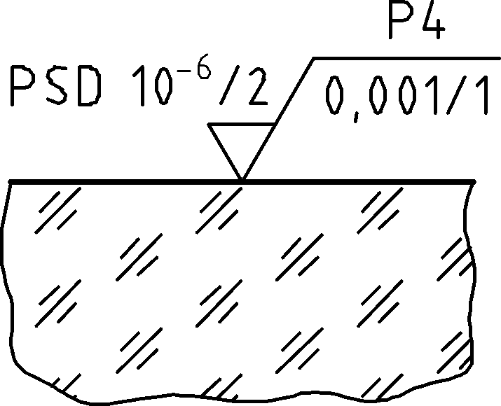. The notation really needs to include a, b, and c coefficients. At a minimum a and b are needed — a coefficient for the power spectrum and then a fractal coefficient. P. Takacs suggested that if the K-Correlation function would be used, then additional slashes would be required after the PSD notation to make room for them. He said that the c parameter indicates the location of the “knee” on the PSD curve. The K-Correlation function is good because it has a finite rms roughness from 0 – ∞. The fractal form has an infinite rms roughness. The a, b, c form can also turn into a fractal function under specific circumstances.

D. Aikens wondered how far from the industry norm this area should be allowed to go. Perhaps a different PSD should be defined, such as PSDK, to permit a different formula for the reporting the power spectrum. P. Takacs suggested that if more numbers were listed after the PSD notation on the indication, then the user would know which form was incorporated.

W. McKinney noted that the majority of PSD curves reported in literature that exhibit the “knee” characteristic are the result of instrumental artifacts. When the three coefficients are added to the indication specified by the standard, then the user may get the impression that the “knees” are a part of the PSD rather than the result of the measurement. If the standard recognizes the “knee” then users may infer that the data in literature showing the knee must be correct.

D. Aikens urged that the straight line portion of the curve is of interest for polished surfaces. The fractal characteristic of the polishing process results in a straight line. P. Takacs agreed with that conclusion for fractal polishing techniques; however, there are cases when the polishing process is not fractal in nature, and some processes can produce plateaus. To illustrate his point, P. Takacs said that a ground surface has a white-noise characteristic. After polishing begins the higher frequencies show attenuation. The rough terrain still shows up in the lower frequencies, but the high frequencies have begun to roll off. That is not a fractal characteristic; rather the PSD looks like the K-Correlation. As polishing continues the high-frequency data levels because its characteristic is limited by the size of the polishing compound. As polishing continues the PSD curve moves toward the left. There is a range of shapes that can be imposed by polishing. J. Harvey added that the K-Correlation does include the fractal condition as a special case.

D. Aikens concluded that the average user will have difficulty understanding any of this. A. Krisiloff reminded the Task Force that the problem is to create a notation that adequately describes what the measurement is to produce. V. Yashchuk pointed out that spatial filtering needs to be considered to take into account the finite pixel size of the detector used to capture the surface data. D. Aikens said that these items would appear in the measurement section (standard for ISO), which still has to be written. M. Dowell asked if the PSD characteristic could be described in the measurement section. D. Aikens replied that what is being proposed is that a user needs to be able to describe a shape, not just a line, for the PSD, and the notation must allow for that. He suggested that the easiest way to accomplish that is to have notations for two different types of PSD. There will probably be four versions altogether:

1. 1D PSD,

2. 2D PSD,

3. 1D PSDK,

4. 2D PSDK.

D. Aikens said that the standard needs default specifications. P. Takacs said that a default would change depending upon the application because different ranges would come into play. D. Aikens replied that the default would be for a typical surface if no scan lengths were specified. P. Takacs continued saying that the default in that case would be the measuring instrument; unfortunately, there is not typical measuring instrument. The measuring instrument for surface roughness traditionally would be a New View or a BAF – an interference microscope with a 10_ objective. S. Martinek said that these instruments are not a default. D. Aikens clarified his assertion that there needs to be a default by saying that the notation should provide a statement telling the optics maker what the lack of a specification means. P. Takacs countered that the notation requires the specification writer to declare a band width.

A. Krisiloff said that he agreed with D. Aikens desire for default specifications, because a standard is better when it offers default conditions. If the standard does not provide for defaults, then there can be instances when a court room would have to decide what the defaults would be.

P. Takacs continued saying that when the user puts the symbol on the drawing, the absence of the bandwidth indication under the check mark raises a flag to the manufacturer. D. Aikens reminded the Task Force that the PSD indication will appear on a small percentage of drawings. In the majority of drawings 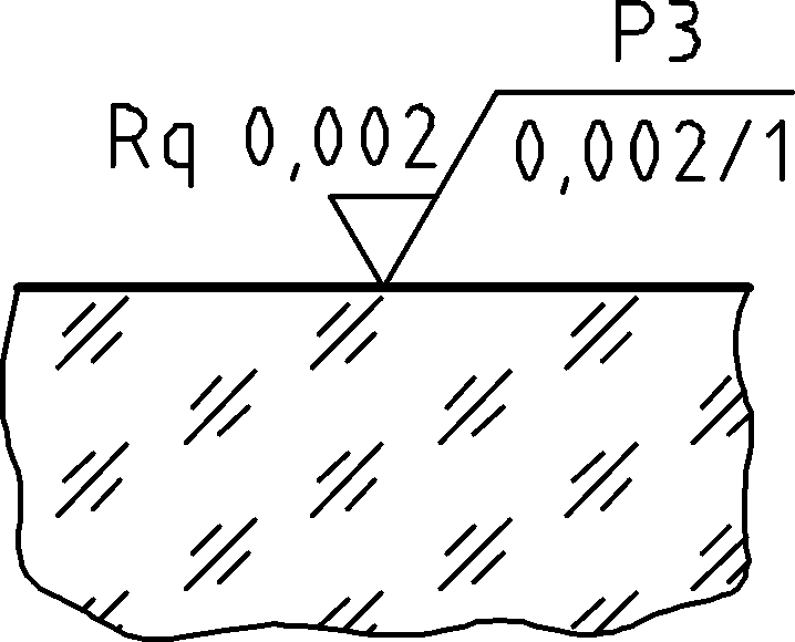is the symbol that will be used, and a lot of engineers write Rq and a value, but they do not include the bandwidth, even though they should. D. Aikens wants the standard to provide a default bandwidth for the manufacturer to use if the engineer forgot to include it. He agreed with P. Takacs in that there should not be a default for PSD.

Tasks to be Completed

At this point S. Martinek asked the Task Force to return to the list of tasks that need to be completed, so that volunteers could be recruited.

• Reconciliation of definitions with ISO/DIS 25178-2 and ASME B46.1 — there could be a table in an annex that cross-references definitions; that was a common practice before different bodies started agreeing on common terms. C. Evans had volunteered to help with this task in conjunction with P. Takacs and D. Aikens. D. Aikens said that he would concentrate on ISO/DIS 25178-2. M. Dowell volunteered to contact Ted Vorburger to get information concerning ASME B46.1.

• Address micro-defects (defined both in 3.4 and 3.14) — S. Martinek suggested that this topic be deemphasized.

• Expanded 2D PSD definitions — P. Takacs, L. Assoufid, V. Yashchuk, W. McKinney

• D. Aikens volunteered to write discussion about rms, rms slope,PSD in the foreword.

• Slope — P. Takacs, L. Assoufid, V. Yashchuk, W. McKinney

• Structure measurement

• Bandwidth limits — D. Aikens, S. Martinek

S. Martinek called for the first draft of the revision for the January meeting. D. Aikens proposed a conference call on November 15, 1:00 pm EST to review interim progress.

The Task Force agreed to add a peak to valley discussion to the January agenda. A review of the OP1.004 draft would also be included.

L. Endelman complemented the Task Force saying that he had seen more progress at this meeting then he had seen in the previous two years. He could almost see the glimmer of a CD coming out.

OP1.005

Not addressed.

6. Time and Place for next OP1 Wavefront Meeting

D. Aikens moved that the group meet next in San Jose, CA on Sunday, January 20, 2008, 2:00 p.m. – 5:00 p.m.. M. Dowell seconded the motion. The motion carried unanimously.

7. Adjournment

D. Aikens moved that the meeting be adjourned. L. Endelman seconded the motion. The meeting was adjourned at 12:03 p.m.